Difference between revisions of "Understanding satnogs-flowgraphs"
Matburnham (talk | contribs) |
Matburnham (talk | contribs) (Sample rate calculation workings - raw, probably needs a tidy-up) (Tag: Visual edit) |
||
| Line 1: | Line 1: | ||
| − | I'm not entirely sure where to put this, but perhaps someone more experienced can move and link this from a sensible location. This started as a question continuing the [https://community.libre.space/t/how-to-open-satnogs-iq-dat-files/3793 How to open satnogs iq.dat files] thread but as I worked through after picking things up after initially having a problem I realised everything I'd described now magically worked! Typical. Worth documenting. | + | ''I'm not entirely sure where to put this, but perhaps someone more experienced can move and link this from a sensible location. This started as a question continuing the [https://community.libre.space/t/how-to-open-satnogs-iq-dat-files/3793 How to open satnogs iq.dat files] thread but as I worked through after picking things up after initially having a problem I realised everything I'd described now magically worked! Typical. Worth documenting.'' |
==Setting yourself up== | ==Setting yourself up== | ||
| Line 32: | Line 32: | ||
===Feeding your IQ in=== | ===Feeding your IQ in=== | ||
| − | Loading the flowgraph in requires some GNU Radio modules chaining together. Starting with [https://community.libre.space/t/how-to-open-satnogs-iq-dat-files/3793 How to open satnogs iq.dat files] you'll end up with something like | + | Loading the IQ into beginning of the flowgraph in requires some GNU Radio modules chaining together. Starting with [https://community.libre.space/t/how-to-open-satnogs-iq-dat-files/3793 How to open satnogs iq.dat files] you'll end up with something beginning like the below. It takes the file source, throttles the output to real-time, then converts the short values to complex real including reversing the scaling division. This feeds then into the existing flowgraph exactly where it left off. |
[[File:flowgraph_open.png|800px]] | [[File:flowgraph_open.png|800px]] | ||
| − | It took some time for me to work out the appropriate | + | === Sample rate === |
| + | It took some time for me to work out the appropriate sample rate. Here's my methodology: | ||
| − | The | + | The IQ recording is generated by the flowgraph in use. If there's no particular decoder in use then that's <code>GNURADIO_DEFAULT_SCRIPT_FILENAME</code> (see [https://gitlab.com/librespacefoundation/satnogs/satnogs-client/-/blob/master/satnogsclient/settings.py#L66 <code>settings.py</code>] as it keeps changing in HEAD - <code>satnogs_fsk_ax25.py</code>, then <code>fsk.grc</code> and now <code>fm.grc</code>). The flowgraph can vary, but it's probably fairly similar for each on the front end. |
| + | |||
| + | From <code>fsk.grc</code>: | ||
| + | |||
| + | # Soapy Source collects data at <code>samp_rate_rx</code>. | ||
| + | # Doppler Compensation takes <code>samp_rate_rx</code> and aims for a Target Sampling Rate of <code>baudrate*decimation</code> (in <code>fsk.grc</code>) or <code>audio_samp_rate</code> (in <code>fm.grc</code>). One assumes these should normally be identical, but perhaps someone brighter can explain the difference and how Doppler Compensation converts - decimation? | ||
| + | # IQ sink stores the data to <code>iq_file_path</code>, with a scaling factor of <code>16768</code> applied. | ||
| + | |||
| + | |||
| + | '''Where do these parameters come from?''' | ||
| + | |||
| + | All jobs come via [https://gitlab.com/librespacefoundation/satnogs/satnogs-client/-/blob/master/satnogsclient/scheduler/tasks.py#L47 scheduler/tasks.py]. This grabs scheduled jobs from the Satnogs network. In JSON format, this looks something like this: | ||
| + | |||
| + | <code>[</code> | ||
| + | |||
| + | <code> {</code> | ||
| + | |||
| + | <code> "id": 2164959,</code> | ||
| + | |||
| + | <code> "start": "2020-05-06T18:53:17Z",</code> | ||
| + | |||
| + | <code> "end": "2020-05-06T19:00:30Z",</code> | ||
| + | |||
| + | <code> "ground_station": 1450,</code> | ||
| + | |||
| + | <code> "tle0": "0 METEOR M2",</code> | ||
| + | |||
| + | <code> "tle1": "1 40069U 14037A 20126.65202808 -.00000042 00000-0 13670-6 0 9996",</code> | ||
| + | |||
| + | <code> "tle2": "2 40069 98.5071 165.7965 0006707 53.4504 306.7289 14.20671999302133",</code> | ||
| + | |||
| + | <code> "frequency": 137100000,</code> | ||
| + | |||
| + | <code> "mode": "LRPT",</code> | ||
| + | |||
| + | <code> "transmitter": "CojkGDaq3u42nRdLdfczng",</code> | ||
| + | |||
| + | <code> "baud": 80000</code> | ||
| + | |||
| + | <code> },</code> | ||
| + | |||
| + | <code> {</code> | ||
| + | |||
| + | <code> "id": 2164887,</code> | ||
| + | |||
| + | <code> "start": "2020-05-06T15:51:13Z",</code> | ||
| + | |||
| + | <code> "end": "2020-05-06T16:06:30Z",</code> | ||
| + | |||
| + | <code> "ground_station": 1450,</code> | ||
| + | |||
| + | <code> "tle0": "0 NOAA 19",</code> | ||
| + | |||
| + | <code> "tle1": "1 33591U 09005A 20126.94623650 +.00000063 +00000-0 +59678-4 0 9999",</code> | ||
| + | |||
| + | <code> "tle2": "2 33591 099.1965 131.1873 0013769 190.9197 169.1677 14.12406430579135",</code> | ||
| + | |||
| + | <code> "frequency": 137100000,</code> | ||
| + | |||
| + | <code> "mode": "APT",</code> | ||
| + | |||
| + | <code> "transmitter": "kE4VaYKpnFmzEquEjKKi8D",</code> | ||
| + | |||
| + | <code> "baud": null</code> | ||
| + | |||
| + | <code> }</code> | ||
| + | |||
| + | <code>]</code> | ||
| + | |||
| + | Clearly, there's no sample rate in that blob, but there is a mode and a baudrate. | ||
| + | |||
| + | |||
| + | '''How do these parameters get to the flowgraph?''' | ||
| + | |||
| + | <code>exec_gnuradio</code> in [https://gitlab.com/librespacefoundation/satnogs/satnogs-client/-/blob/master/satnogsclient/upsat/gnuradio_handler.py#L60 satnogsclient/upsat/gnuradio_handler.py#L60] takes all the parameters collected and passes them as command line arguments to the relevant flowgraph. It looks like the samp-rate-rx comes from SATNOGS_RX_SAMP_RATE in settings.py. | ||
| + | |||
| + | |||
| + | '''So where does the sample rate actually come from!?''' | ||
| + | |||
| + | Ah, it looks like it's actually static and stored in /etc/ansible/host_vars/localhost: | ||
| + | |||
| + | <code>...</code> | ||
| + | |||
| + | <code>satnogs_rx_samp_rate: 2.048e6</code> | ||
| + | |||
| + | <code>...</code> | ||
| + | |||
| + | So it's a static sample rate regardless of flowgraph. Okay, that might explain why the Doppler Compensation has different output sample rate and does some kind of decimation. | ||
| + | |||
| + | ''Note: it looks like the new fm.grc doesn't pass a baudrate - what effect will this have on things like LPRT that don't have their own flowgraph handled at present?'' | ||
| + | |||
| + | '''Summary''' | ||
| + | |||
| + | The key value is the Doppler Compensation ''Target Sampling Rate''. | ||
| + | |||
| + | For the simple case of APT imaging through [https://gitlab.com/librespacefoundation/satnogs/satnogs-flowgraphs/-/blob/master/satellites/noaa_apt_decoder.grc noaa_apt_decoder.grc] this is pretty simple. it's a static value 4*4160*4 or 66,560. | ||
| + | |||
| + | It's a more complicated case for say an LRPT signal from [https://db.satnogs.org/satellite/40069/ METEOR M2] for example. This runs through <code>satnogs_fsk_ax25.py</code> at least in my live system. One needs to look at the database page and get the Baud rate of the relevant transmitter (80,000 in this case). Then look at the Doppler Compensation ''Target Sampling Rate'' again which turns out to be <code>baudrate*decimation</code>. Argh! Decimation turns out to be <code>max(4,satnogs.find_decimation(baudrate, 2, audio_samp_rate))</code>. So what's <code>audio_samp_rate</code>? Luckily it's static and set in <code>satnogs_fsk_ax25.py</code> to <code>48e3</code>. | ||
| + | |||
| + | Using gr-satnogs/python/utils.py, this is easy to calculate: | ||
| + | |||
| + | <code>>>> import utils as satnogs</code> | ||
| + | |||
| + | <code>>>> baudrate = 80000</code> | ||
| + | |||
| + | <code>>>> audio_samp_rate = 48000</code> | ||
| + | |||
| + | <code>>>> max(4,satnogs.find_decimation(baudrate, 2, audio_samp_rate))</code> | ||
| + | |||
| + | <code>4</code> | ||
| + | |||
| + | So, by my calculation, my IQ should be at 4 * 80,000 = 320,000. Hopefully. | ||
| + | |||
| + | '''Alternative route''' | ||
| + | |||
| + | After all this hassle, I think the easy fix is the put in a pre-observation script to dump to the logfile! Looks like the following will give me most of what I need, although I'll still need to do some maths. | ||
| + | |||
| + | <code>echo <nowiki>{{ID}}</nowiki> <nowiki>{{BAUD}}</nowiki> <nowiki>{{SCRIPT_NAME}}</nowiki></code> | ||
===Results=== | ===Results=== | ||
Revision as of 16:19, 6 May 2020
I'm not entirely sure where to put this, but perhaps someone more experienced can move and link this from a sensible location. This started as a question continuing the How to open satnogs iq.dat files thread but as I worked through after picking things up after initially having a problem I realised everything I'd described now magically worked! Typical. Worth documenting.
Contents
Setting yourself up
See elsewhere, but get GNU Radio up and running and a copy of satnogs-flowgraphs from GitLab.
I'm using a virtual Ubuntu 19.10 machine grabbed from osboxes.org, but you can use whatever you like. I imagine you could even do it on the Raspberry Pi itself. I did end up setting this VM up as a 'development station' but you should only need to install GNU Radio, and any pre-requisites needed by satnogs-flowgraphs - so probably gr-satnogs, I can't quite remember. As you find out please edit this :-)
Storing an IQ recording
There are options in satnogs-setup under Advanced > Radio to store IQ files:
- ENABLE_IQ_DUMP: Enable IQ dump
- IQ_DUMP_FILENAME: Define IQ dump filename [/tmp/.satnogs/iq.raw]
Beware, IQ files are huge (220MB for my APT pass example below). They're stored in /tmp so therefore in RAM and are overwritten with each pass. You can do something clever to upload them elsewhere, but for playing just grab a copy immediately after a pass.
Don't worry about storing much else (which also vanishes quickly). You can easily grab waterfalls and OGG recording from the database via Glouton.
GNU Radio Companion
Here I'm working with Observation #2073316 as an example. I've saved a copy of the IQ recording my station briefly stored at `/tmp/.satnogs/iq.raw`. This is about 220 MB. I even remembered to turn the IQ collection off afterwards or it would be storing stuff on top of each other forever.
So where did the IQ come from?
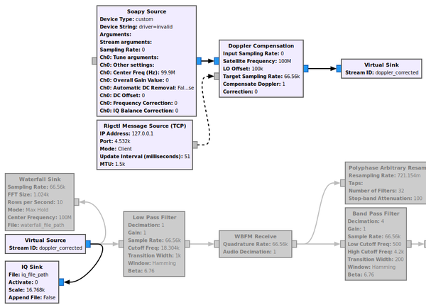
In my case, I'm playing with an APT pass. It is therefore processed by satnogs-flowgraphs/satellites/noaa_apt_decoder.grc. Other signals use other flowgraphs. The default where nothing else is suitable appears to be satnogs-flowgraphs/generic/fsk.grc.
That is, it's post Doppler correction, which includes an LO offset; and the values are scaled to shorts, although 16768 seems an weird number as I'd have expected a power of two - 16384? I don't imagine it makes a lot of difference as it'll still fit in the short just lose a little bit of dynamic range.
Feeding your IQ in
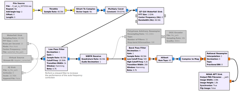
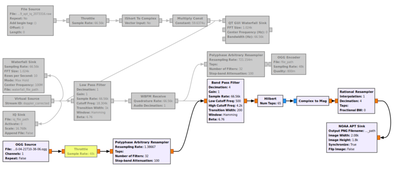
Loading the IQ into beginning of the flowgraph in requires some GNU Radio modules chaining together. Starting with How to open satnogs iq.dat files you'll end up with something beginning like the below. It takes the file source, throttles the output to real-time, then converts the short values to complex real including reversing the scaling division. This feeds then into the existing flowgraph exactly where it left off.
Sample rate
It took some time for me to work out the appropriate sample rate. Here's my methodology:
The IQ recording is generated by the flowgraph in use. If there's no particular decoder in use then that's GNURADIO_DEFAULT_SCRIPT_FILENAME (see settings.py as it keeps changing in HEAD - satnogs_fsk_ax25.py, then fsk.grc and now fm.grc). The flowgraph can vary, but it's probably fairly similar for each on the front end.
From fsk.grc:
- Soapy Source collects data at
samp_rate_rx. - Doppler Compensation takes
samp_rate_rxand aims for a Target Sampling Rate ofbaudrate*decimation(infsk.grc) oraudio_samp_rate(infm.grc). One assumes these should normally be identical, but perhaps someone brighter can explain the difference and how Doppler Compensation converts - decimation? - IQ sink stores the data to
iq_file_path, with a scaling factor of16768applied.
Where do these parameters come from?
All jobs come via scheduler/tasks.py. This grabs scheduled jobs from the Satnogs network. In JSON format, this looks something like this:
[
{
"id": 2164959,
"start": "2020-05-06T18:53:17Z",
"end": "2020-05-06T19:00:30Z",
"ground_station": 1450,
"tle0": "0 METEOR M2",
"tle1": "1 40069U 14037A 20126.65202808 -.00000042 00000-0 13670-6 0 9996",
"tle2": "2 40069 98.5071 165.7965 0006707 53.4504 306.7289 14.20671999302133",
"frequency": 137100000,
"mode": "LRPT",
"transmitter": "CojkGDaq3u42nRdLdfczng",
"baud": 80000
},
{
"id": 2164887,
"start": "2020-05-06T15:51:13Z",
"end": "2020-05-06T16:06:30Z",
"ground_station": 1450,
"tle0": "0 NOAA 19",
"tle1": "1 33591U 09005A 20126.94623650 +.00000063 +00000-0 +59678-4 0 9999",
"tle2": "2 33591 099.1965 131.1873 0013769 190.9197 169.1677 14.12406430579135",
"frequency": 137100000,
"mode": "APT",
"transmitter": "kE4VaYKpnFmzEquEjKKi8D",
"baud": null
}
]
Clearly, there's no sample rate in that blob, but there is a mode and a baudrate.
How do these parameters get to the flowgraph?
exec_gnuradio in satnogsclient/upsat/gnuradio_handler.py#L60 takes all the parameters collected and passes them as command line arguments to the relevant flowgraph. It looks like the samp-rate-rx comes from SATNOGS_RX_SAMP_RATE in settings.py.
So where does the sample rate actually come from!?
Ah, it looks like it's actually static and stored in /etc/ansible/host_vars/localhost:
...
satnogs_rx_samp_rate: 2.048e6
...
So it's a static sample rate regardless of flowgraph. Okay, that might explain why the Doppler Compensation has different output sample rate and does some kind of decimation.
Note: it looks like the new fm.grc doesn't pass a baudrate - what effect will this have on things like LPRT that don't have their own flowgraph handled at present?
Summary
The key value is the Doppler Compensation Target Sampling Rate.
For the simple case of APT imaging through noaa_apt_decoder.grc this is pretty simple. it's a static value 4*4160*4 or 66,560.
It's a more complicated case for say an LRPT signal from METEOR M2 for example. This runs through satnogs_fsk_ax25.py at least in my live system. One needs to look at the database page and get the Baud rate of the relevant transmitter (80,000 in this case). Then look at the Doppler Compensation Target Sampling Rate again which turns out to be baudrate*decimation. Argh! Decimation turns out to be max(4,satnogs.find_decimation(baudrate, 2, audio_samp_rate)). So what's audio_samp_rate? Luckily it's static and set in satnogs_fsk_ax25.py to 48e3.
Using gr-satnogs/python/utils.py, this is easy to calculate:
>>> import utils as satnogs
>>> baudrate = 80000
>>> audio_samp_rate = 48000
>>> max(4,satnogs.find_decimation(baudrate, 2, audio_samp_rate))
4
So, by my calculation, my IQ should be at 4 * 80,000 = 320,000. Hopefully.
Alternative route
After all this hassle, I think the easy fix is the put in a pre-observation script to dump to the logfile! Looks like the following will give me most of what I need, although I'll still need to do some maths.
echo {{ID}} {{BAUD}} {{SCRIPT_NAME}}
Results
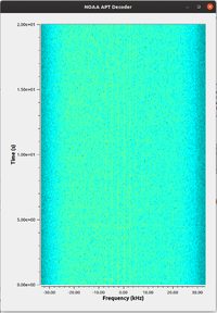
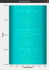
Initially, the waterfall may look a bit busy compared to the one from the observation. There's obviously some gain setting within the waterfall I've not yet mastered, or the Satnogs ones does something slightly cleverer.
Yep. It turns out you can set the intesity min and max to better reflect the signal and get a cleaner display. Still not as good as the observation page one, but maybe that fiddles with the FFT size too.
However, if you peer closer you can just about make out the feint telltales of an APT signal.
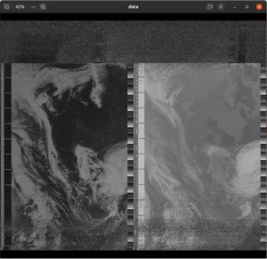
Following the flowgraph through to output shows an identical output to that on the observation. Result!
OGG
For completeness, you can do the same thing using the OGG file as a source. Again, you need to reverse any resampling or other changes that were done before saving to file before feeding back into the flowgraph at an appropriate point. The throttle is optional, and in the screenshot bypassed:
